Cable Equation Model

This is the second write-up where I'll be documenting my research with Dr. Joyce Lin. If you want to read my introductory article regarding the research series, you can check it out here.

Introduction

The cable equation was first synthesized by Lord Kelvin (formerly William Thomson) in 1855; he derived the cable equation to study the signal decay in the transatlantic telegraph cable (then under construction). His foundational work would become extremely valuable in the realm of neuronal behavior mainly due to Hodgkin and Ruston in 1946 which was then followed by a series of papers by Rall. [1]

Equation

The equation itself is as follows:

After nondimensionalizing, it reaches a simpler equation like this:

Here, $X$ and $T$ are non-dimensional variables each of which individually represents $X = x / \lambda_m$ and $T = t / \tau_m$. Also, $\lambda_m$ represents the membrane space constant and $\tau_m$ represents the membrane time constant. The $f$ corresponds to a function that accounts for the ionic channels that exist through the cell membrane. For our simulation, we use the Hodgkin-Huxley Equations to generate the ionic current, i.e., $I_{ion} = -f(V, t) R_m$. Here $R_m$ is our membrane resistivity.

At its core, the cable equation provides us with a framework where one can analyze the spatial distribution of electric pulses. The capacitance of the outer insulator or "membrane" leads to the temporal and spatial differences in voltage or "transmembrane voltage".

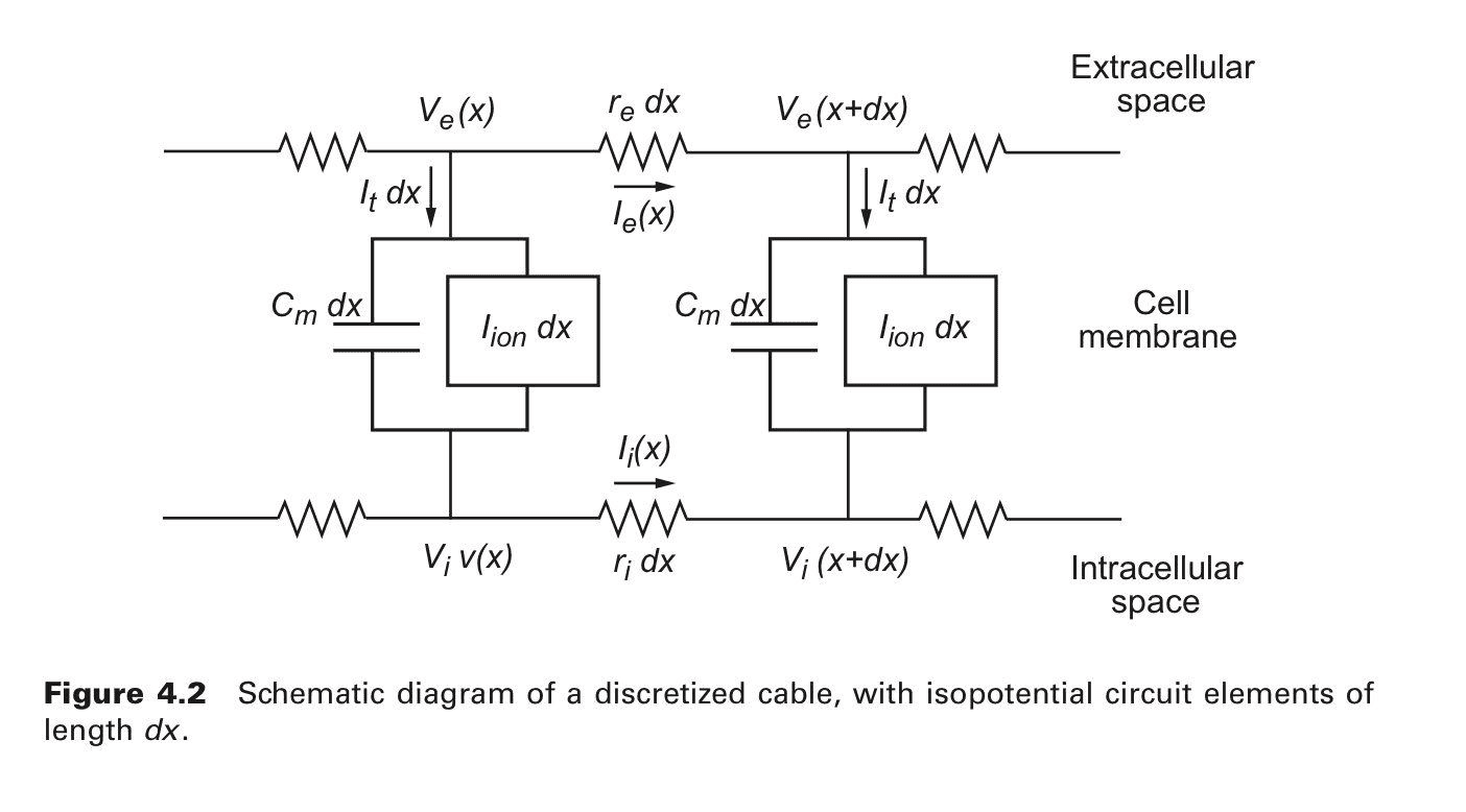Cable equation schema diagram Representation of Cable Model at a cellular level [2]

Assumptions required for the Cable Equation Model

While the model itself is our first true attempt at reasoning the conduction of the action potential, it's still far from a complete explanation. Namely, due to a few key assumptions we make to derive our equation:

• The cable is linear, constant, and infinitely long cylinder.
• The current flow is defined along the length of the cable ($V = V(x, t)$).
• We disregard radial or angular variables thus allowing us to expect the potential to be uniform when moving radially. This assumption is known as the core conductor assumption.

The resistance from the extracellular and intracellular conductor/space ($r_e$ and $r_i$ in $\Omega \cdot cm$) is:

Here $rad$ is the radius of the cross-section of the cylinder.

The membrane parameter $C_m$ is constant and does not depend on the transmembrane potential.

Simulation

Considering all of the above assumptions, I was able to model the behavior of the action potential as it traverses through the "strand" of cardiac tissue. The simulation below is an animation of multiple snapshots in time (in seconds) of the transmembrane potential (in mV) vs length of the strand (in cm). The simulation itself was coded up using Python and related libraries. To view the code behind the simulation, click here.

The entire source code is available here.

Citations

[1] Douglas, PK; Douglas, DB (2019). "Reconsidering Spatial Priors In EEG Source Estimation: Does White Matter Contribute to EEG Rhythms?". 7th International Winter Conference on Brain-Computer Interface (BCI), Gangwon, Korea (South): 1-12. doi:10.1109/IWW-BCI.2019.8737307.

[2] Keener, Sneyd, and Sneyd, James. Mathematical Physiology: I: Cellular Physiology. 2nd Ed. 2009. ed. New York, NY: Springer New York: Imprint: Springer, 2009. Interdisciplinary Applied Mathematics, 8/1. Web.